More than one clock
A series advances on a single axis (a chart, in charting) — its bars, its ticks, its bricks — and for a while that is all you think about. Then the question changes shape. You want to compare the current price to where the daily average sits. You want a Renko series and a candlestick series to be the same analysis, not two engines. You want to overlay another asset that trades on its own calendar, or to add three calendar months to an expiry across a daylight-saving boundary. Every one of those is the same move: relating your series to another clock.
This chapter is about that move, and it turns on the same idea as the last chapter: a clock in
Flux is not a hidden setting — it is a value, with a kind, that flows through if and def and
input like any other. Once the step axis is a
value you can choose it, pass it, and read one series as of another, and the whole family of
“different resolutions” and “different geometries” collapses into one small idea. By the end you
will resample an indicator onto the daily clock in one operator, pull in a second asset without
breaking replay, do honest calendar arithmetic, and watch the forming unit (the forming bar, in charting) develop on screen
without ever letting it touch a number.
The clock is a value
Start with the plain idea: a clock is the rule that decides when one step ends and the next begins — and in Flux it is a value you hold, not a setting buried in a menu.
Every series advances on a clock, and clock is a first-class kind: an ordinal step index
paired with a mapping between step indices and time. A clock answers exactly two questions —
what is step i’s timestamp? and which step contains time t? — and nothing more. Position
on the axis is always the ordinal step index, never wall-time; the clock is what translates
between the two.
Four constructors build one:
| constructor | steps advance on | example |
|---|---|---|
tf("1h") |
closed time buckets | hours, days, weeks |
renko(box) |
price moving one box : level |
bricks |
pnf(box, rev) |
price filling boxes, reversing after rev |
point-and-figure columns |
range(r) |
price traversing a range r |
range bars |
The row that matters most is the one your eye skips: time-coarse clocks and price-driven clocks are the same concept — a rule for when a unit closes. That single fact pays for itself twice. It means a Renko or point-and-figure series is not a renderer bolted onto the base series’ data (bar data, in charting); it is the ordinary series machinery running on a different clock. And it means multi-resolution analysis is not a special feature: an expression “at another resolution” is just an expression on another clock, read back onto yours.
Because a clock is an ordinary value, it goes wherever values go — through a branch, a function
parameter, an input:
regime = adx(14).adx > 25                     // signal — a trending regime
c      = if regime then tf("1d") else tf("4h") // clock — chosen like any other value
Constructor parameters const-fold, exactly as a delay index or a window capacity does:
renko(50) (the literal adopts kind level), or a bounded input. A data-dependent box is
rejected — a clock is a fixed axis, not a quantity that drifts with the data it is supposed to
index. Clocks also flow into functions: barsPerYear(clk) derives the periods-per-year of a
time clock for annualization, and on an event clock (renko, pnf) — where the question has no
answer — it returns na with a diagnostic rather than a fiction.
Reading another clock: @
Choosing a clock is half the story; the other half is reading a value computed on it back onto
your own steps. That is the postfix @ operator, and it is the one operation that consumes a
clock — the eliminator of the clock kind. e @ c evaluates e per unit of clock c and
reads the result on the current series’ steps:
c   = tf("4h")                                // clock — a first-class value
d   = ema(close, 20) @ "1d"                   // price — the daily EMA, on the chart's steps
r   = rsi(close, 14) @ tf("1h")               // osc(0,100) — kind-preserving
x   = close @ c                               // any clock value works as the operand
Two properties make @ trustworthy. It is kind-preserving (resample : (α, clock) → α) —
a daily EMA is still a price, an hourly RSI still an osc(0,100) — so resampling never quietly
changes what a value means. And it is causal: at any step, e @ c reads the value of e at
the last closed unit of c, never the one still forming. The forming unit is exactly the
value that will still change, and letting analysis read it would manufacture the repaint the whole
language exists to exclude.
@ binds tighter than comparison, which is what makes the everyday confluence idiom read the
way you say it out loud:
plot close > ema(close, 20) @ "1d" // signal — close vs the last CLOSED daily EMAThis parses as close > (ema(close, 20) @ "1d"): the current step’s close against the daily
average as of the most recent completed day. The operand may be a string literal (shorthand for
the time-coarse clock it names), an identifier or a call (tf("1h"), renko(box)), or a
parenthesized expression.
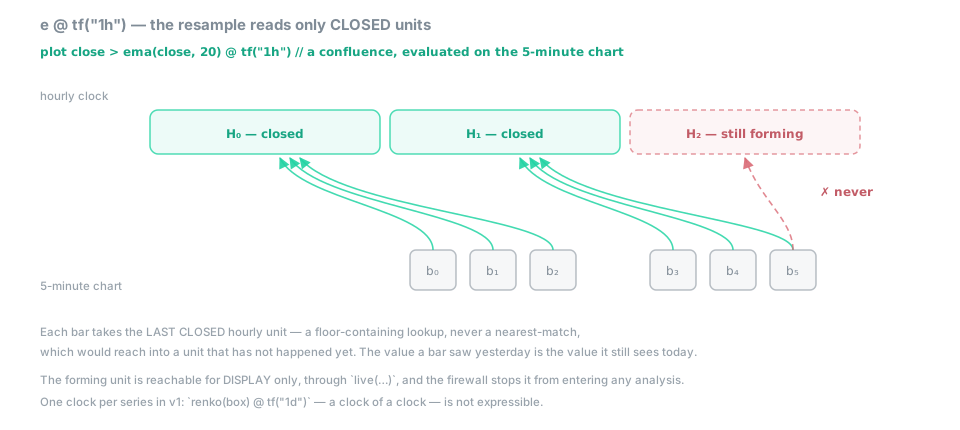 Figure —
 e @ tf("1h"): every fine step reads the last closed coarser unit; the forming unit is invisible to analysis, and steps before the first closed unit read na.
The alignment that makes this causal is floor-containing: a step whose time is t maps to the
coarser unit whose span contains t — the most recent one whose start is Tₖ ≤ t — and then reads
the last unit already closed. It is deliberately not round-to-nearest, because rounding a step in
the first half of a forming unit to that forming unit reads data that did not exist yet, and
history would repaint when the unit closed. Floor-containing is the one alignment under which
output[t] = f(inputs[0..t]) survives resampling. Before the first closed coarser unit, e @ c
is na — resampling inherits warm-up like everything else.
One clock per series
Here is the honest limit, stated as plainly as the feature. A series has exactly one clock, so a clock cannot be resampled onto another clock:
close @ renko(50) @ "1d" // ✗ — one clock per series in v1: no clock compositionStacked re-bucketing — price bricks, then a daily aggregation of the bricks — is a coherent idea
and deliberately outside the sealed scope of this version. @ reads one coarser clock onto your
own; it does not chain clocks. The full contract that @ obeys — position is ordinal, the locator
is floor-containing, only closed units are readable, byte-identity holds through the resample — is
pinned by a set of invariants in the spec, linked below.
Foreign series: the as-of join
Resampling is one case of a more general problem: aligning a series that closes on its own
schedule onto your ordinal axis. Another asset, another venue, another session calendar — their
steps do not land where yours do. The rule that lines them up is the as-of join, and it is the
same floor-containing rule as @, said for foreign data:
At chart step
t, a foreign series reads its most recent step with timestamp ≤t’s time.
Never round-to-nearest — that would peek at a foreign step that had not happened yet. During a
foreign gap (its market closed while yours is open) the value holds: the last known foreign
value is still the most recent one. Before the first foreign step it is na, ordinary warm-up.
eth = series("ETH-USD").close // price[ETH,USD] — aligned as-of, holds over gaps
rel = close / eth // ratio — cross-rate (same quote), plottable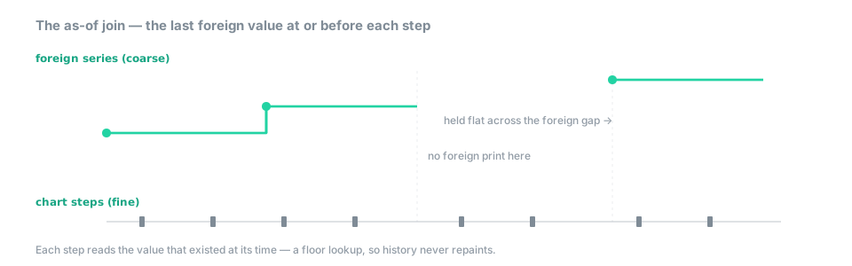 Figure — the as-of join: each chart step takes the last foreign value at or before its time, and holds it across the foreign gap.
Because the as-of join admits no future row, the no-repaint property carries over untouched: a
cross-series indicator is exactly as replayable as a single-series one. What you may combine is
guarded separately by the kind system — the asset and currency tags on price make
price[BTC,USD] + price[ETH,USD] an [ErrDim], which the cross-rate above sidesteps because a
division cancels the shared quote. That algebra lives in
FDK — Asset & currency, and the windowed asofJoin primitive in
FDK — Compute.
Time itself: points, durations, periods
The as-of rule leans on timestamps, and time in Flux carries the same affine discipline as the price axis — a point is not a displacement, and the two do not add. Three kinds make that concrete:
| kind | role | representation |
|---|---|---|
time |
a point on the timeline | machine instant (64-bit epoch) |
duration |
a vector of elapsed machine time | exact — machine tag |
period |
a vector of calendar time | zone/DST-aware — calendar tag |
duration and period are the same dimensional object — a displacement on the time axis —
distinguished by a representation tag, exactly as f64 and decimal tag the same numeric
dimension. Both add to a point to give a point:
age    = time - time[1]                       // duration — pt(T) − pt(T) → vec(T), exact
expiry = time + time.months(3)                // time — calendar arithmetic, DST-aware
later  = time + time.months(1) + time.days(10)   // period constructors compose
period values come only from the calendar constructors — time.years(n), time.months(n),
time.weeks(n), time.days(n), on const arguments — and the two representations never mix
implicitly:
time.days(1) + (time - time[1]) // ✗ [ErrRepr] — calendar + machine: convert explicitlyThe error is doing you a favour. “One day” and “24 hours” are different claims: across a
daylight-saving transition, adding time.days(1) lands on the same wall-clock time the next civil
day, while a 24-hour duration lands an hour off. Both are useful; silently conflating them is
how session logic breaks twice a year, so the tag makes the conversion a visible decision. The
calendar accessors — year, month, day, hour, minute, second, dayOfWeek, dayOfYear
— project a time into a declared zone and return num; because they run in the ANALYSIS plane,
that zone is a pinned replay input, never an ambient per-viewer setting, so two machines never
disagree on the same script. Arithmetic that leaves the representable range does not wrap — it
yields na with a diagnostic, keeping timestamps in causal order. The exhaustive calendar
algebra — every constructor, the zone model, the representable range — is pinned in
Points, durations and periods.
The forming unit: live()
Everything so far concerns confirmed values — streams that advance when a unit closes, and
that @ reads only after the fact. A display legitimately wants one more thing: the unit still
forming, updating tick by tick. live(e) provides it, as a presentation value, and it is the
mirror image of the closed-unit rule — where @ reads the last closed unit, live reaches into
the one still open.
plot live(ema(close, 20))                     // ✓ display — the forming step included, per frame
h1  = high @ live(tf("1h"))                   // ✓ display — the forming hour's running high

rsi(live(close), 14)                          // ✗ [ErrFirewall] — feeding an analysis calculation
alert live(close) > sma(close, 20)            // ✗ [ErrFirewall] — alerts are confirmed sinks
assert live(close) > 0                        // ✗ [ErrFirewall] — assertions run on confirmed data
live(e) re-evaluates the analysis sub-graph of e per frame, including the forming unit, and it
is kind-preserving (κ(live(e)) = κ(e)). Wrapping the clock instead — high @ live(tf("1h")) —
scopes the liveness to the resample, so only the coarser clock’s forming unit is read live while
everything else stays confirmed. The one rule is a boundary: a live(…) value may flow only into
display sinks — plot, mark, fill, color bars, a scene. The firewall bars every confirmed
sink, because feeding the forming unit into a calculation, an alert, or an assertion would
manufacture exactly the repaint the language excludes — an indicator that looks prescient live and
rewrites itself at the close.
The trade is exact and worth stating: the confirmed stream of e is byte-identical whether or not
live appears anywhere in the script, so live() values are excluded from the byte-identity
oracle just as wall-clock signals are. A script that uses live() is flagged non-replayable —
its display cannot be reproduced from the journal, because the forming data it painted was never
committed — while its analysis stays fully replayable. The flag is about the pixels, not the
numbers.
Events on the axis
The last piece is the small vocabulary that ties streams to calendars and events on whatever clock
you are on — the everyday helpers are below, while the full catalogue and each helper’s @lag is the spec’s:
| helper | kind | meaning |
|---|---|---|
in_session(spec) |
signal |
1 while the named session is open; the spec names hours, zone and the asset calendar |
barssince(s) |
barspan |
steps elapsed since s last fired |
valuewhen(s, x) |
kind of x |
the value x had when s last fired |
count(s, n) |
osc(0,n) |
how many of the last n steps fired s |
rising(x, n) / falling(x, n) |
signal |
monotone over the last n steps |
a cross_up b / a cross_down b |
signal |
crossing, as an infix comparison |
sess   = in_session("09:30-16:00 America/New_York")   // signal
sinceX = barssince(close cross_up ema(close, 50))    // barspan
atX    = valuewhen(close cross_up ema(close, 50), close)   // price — held until the next firing
Notice barssince returns barspan, not a bare number: a count of steps carries the ordinal
dimension of the x-axis, which is affine too, so a bar count cannot be silently added to a price —
while barindex − barindex → barspan and slope-like quantities (price per barspan) fall out of
the algebra with the right kinds.
The vocabulary earns its keep at the one place hindsight is unavoidable — a pivot, a local extremum, which is not knowable until enough later steps have failed to exceed it. Flux puts that latency in the signature rather than hiding it:
ph  = pivot_high(high, 3, 3)                  // signal @lag 3 — confirmed 3 steps after the top
lvl = valuewhen(ph, high)                     // price — the last confirmed pivot level
The @lag 3 is part of the frozen signature: the signal fires on the step where confirmation
completes, three steps after the extremum, and that delay is documented, bounded and visible — not
an implementation surprise. The familiar alternative, a zigzag whose last leg mutates until the
next pivot confirms, is inexpressible on purpose: a mutating last value is a produced value that
changed (repaint, excluded by causality), and its confirmation latency is unbounded (excluded by
totality). Where you do want the forming leg on screen, you draw it with live() — a provisional
marker that never becomes an analysis value. What cannot be written is precisely the part that
would have lied.
See also
- Guide §4 — Streams, delay and running state — the stream model,
scan, and the causality theorem this chapter resamples over. - Guide §5 — Kinds — the affine kinds
price,level,time,durationandbarspancarry. - Guide §14 — What Flux deliberately doesn’t do — one-clock-per-series and other honest v1 limits.
- Spec — Time & state (Analysis) — the reference semantics narrated above.
- FDK — Compute —
asofJoinand the windowed statistics behind foreign-series alignment. - Guide §13 — Cookbook — worked recipes: multi-resolution confluence, anchored VWAP.
The formal rules →
- Clocks — the step axis as a value, and the four constructors →
@, the clock eliminator — kind-preserving, causal resampling →- The floor-containing locator, and the seven-invariant clock contract (I1–I7, one clock per series) →
- Foreign series and the as-of rule →
- Points, durations and periods — machine vs calendar time →
live(e)— the forming unit, display only →- Session, event and pivot helpers, and pivot
@lag→