Time and state
A value in the ANALYSIS plane is not a number but a history — it advances one step at a time, and everything you can say about it is a statement about that advance. This page specifies that temporal model in full: what a stream is, how the past is reached, why the future is not addressable, how bounded state and iteration are written, and how the step axis of a series — its clock — is itself a first-class value. The guarantees the rest of Flux leans on are defined here: causality (a value depends only on the past), no-repaint (a value, once produced for a step, never changes), totality (every construct terminates within a compile-time bound) and byte-identity (the same program produces the same bytes on every engine, warm-up included).
Kinds (price, level, signal, …) are specified in Kinds; this page uses
them freely and annotates examples with them. The presentation-side clocks — frames and events
— belong to Canvas and The APP plane; the clock here is the
data clock, the one analysis values advance on.
New here? Start with Guide §4 — Streams, delay and running state → — the clock model is retold in Guide §6 — More than one clock.
Everything is a stream
A value in the ANALYSIS plane is a stream: a value-over-steps. close is not a number;
it is the whole history of closing values, one per step of the chart’s clock. A constant is a
degenerate stream — the same value at every step. In the charting specialization a step is a
bar; nothing in the model depends on that reading.
Arithmetic is element-wise: an expression relates entire streams, and the result is again a stream.
fast   = ema(close, 12)      // price — a stream: one value per step
slow   = ema(close, 26)      // price
spread = fast - slow         // level — element-wise: spread at step t = fast[t] - slow[t]
There are no indices to manage and no loops to write: you state the relation once, and it holds at every step. Under the hood the runtime is incremental — when a new step arrives, each node advances by one, reusing its own bounded state; nothing is recomputed from the beginning. The element-wise reading (whole histories) and the incremental one (one step at a time) describe the same program; the compiler owes you their equivalence.
Why this rule exists. Index-free streams are what make the rest of the page possible. Because a program never names positions, it cannot name a future position; because every operator advances step-by-step with bounded state, totality and memory bounds are properties of the language, not of the author’s discipline.
The delay operator x[n]
The only way to reach into the past is the postfix delay x[n]: the value the stream x had
n steps ago.
prev = close[1]              // price — the previous step's close; na on the first step
diff = close - close[1]      // price − price → level : the one-step change
up4  = close > close[4]      // signal — na on the first four steps (comparison propagates na)
Rules:
nis a const-folded constant,n ≥ 0— a literal, or a parameter whose bounded range lets the compiler reserve the worst case. Delay is memory; memory is bounded at compile time.- Before step
n,x[n]isna— the past that does not exist yet (see Warm-up andna). - On a
vec, the same postfix[i]is a bounded element read, not a delay; the kind of the operand disambiguates.
A data-dependent delay is rejected: the lag would be unbounded.
k = barssince(close cross_up open)
close[k] // ✗ [ErrTotal] — the lag must be a compile-time constantThere is no negative index
x[-1] — “the next value” — does not exist. Not as a discouraged form, not as a lint that a
determined author can silence: there is no such form. The delay index is non-negative by
the language definition, and any attempt to write a negative one is rejected.
close[-1] // ✗ [ErrCausal] — the future is not addressableWhy this rule exists. Causality is a compile-time property, not a style rule. In a language where
x[-1]parses and merely warns, every guarantee downstream — replayability, alert trustworthiness, byte-identical re-execution — holds only for well-behaved scripts. Flux inverts the burden: the ill-behaved script is inexpressible, so the guarantees hold for every program that compiles.
Causality is a theorem
Because the past is reachable only through bounded, non-negative delay, and the forming unit
of any clock is unreadable (see @ — the clock eliminator), every
ANALYSIS program satisfies, by construction:
output[t] = f(inputs[0..t])The value at step t is a function of the inputs up to and including step t — never of
anything later. Two consequences follow.
Every feedback cycle passes a unit delay. A definition may depend on its own previous value (that is what running state is), but never on its own current value — a cycle with no delay has no causal reading and is rejected:
ema20 = 0.1 * close + 0.9 * ema20                       // ✗ [ErrCausal] — cycle with no unit delay
ema20 = scan(close, (prev) -> 0.1 * close + 0.9 * prev) // ✓ the delay is built into scan
scan (below) is the sanctioned way to close a feedback loop: the combinator hands you the
previous step’s output, so the unit delay is part of its meaning rather than something you
remember to insert.
No-repaint. Since output[t] depends only on inputs[0..t], and inputs are append-only,
a value once produced can never be contradicted by later data. This is the no-repaint
guarantee: a value, once produced for a step, never changes. History is immutable — the
chart you scroll back to is exactly the chart that was computed live, the alert that fired is
exactly the alert a re-execution fires. Repaint is not “detected” or “warned about”; it is
absent from the vocabulary. The full family of rejections shares one diagnostic:
[ErrCausal] — negative delay, a non-causal resample, a feedback cycle with no unit delay,
an unbounded lag.
Warm-up and na
Most kernels need history before they can answer: a 14-step RSI has nothing honest to say at
step 3. Until enough data has arrived, a kernel’s output is na — the absent value. This is
its natural warm-up, and each kernel inherits exactly the warm-up of its definition; the
language imposes no blanket “na until N” policy on top. Byte-identity holds from the very
first step: a Flux kernel and the host’s native implementation of the same kernel agree on
every byte, warm-up included (invariant I6).
na inhabits every kind (na : ∀κ.κ) and propagates through arithmetic with the kind
preserved. Its comparison semantics are strict:
- Any comparison involving
na—na == x,na < x, evenna == na— isna, nevertrueorfalse. You cannot test absence with==. - Absence is tested with
is_na(x) → signal; presence with its dualis_some(x) = not is_na(x) → signal. matchon a value that may benamust cover it (annaarm or_), or the match is rejected as non-exhaustive.- Destructuring an absent record (
let {upper, lower} = bbwhenbbisna) givesnain every field.
r     = rsi(close, 14)       // osc(0,100) — na on steps 0..13
warm  = is_na(r)             // signal — 1 during warm-up
bad   = r == na              // na, always — never true; use is_na
assert r <= 100              // passes from step 0: na <= 100 is na, and an na verdict is PASS
The assert verdict on na is deliberately pass: an assertion fires only on a signal that
is definitively false, so warm-up cannot produce spurious failures. Where absence itself must
fail, write assert is_some(r) and r <= 100.
Substitution of a default uses nz(x, d), or its operator form x ?? d (they are the same
construct):
o  = nz(obv(), 0)            // volume — 0 is a literal and adopts the slot's kind
f  = close ?? sma(close, 5)  // price — x ?? d ≡ nz(x, d); right-associative
Both operands must agree dimensionally (the result kind is their join); same dimension with
different representation tags — f64 against decimal, machine time against calendar time —
is [ErrRepr], asking for an explicit conversion.
Absorption vs propagation. Arithmetic propagates na. Three pointwise operators absorb
it instead — math.max, math.min, nz — so math.max(x, na) = x: a missing operand does not poison a
running extreme. Window reducers do not inherit that absorption: highest(x, 20) over a
window containing a hole yields na, exactly as sma, sum and stdev do. The asymmetry is
pinned by byte-identity to the host kernels: the window reducers follow the native oracle, and
a hand-written fold with max (which skips na by absorption) is a different — legitimate —
program, not a faster spelling of highest.
One representation note: na is a single pinned bit pattern at every storage and hashing
boundary, so that byte-identity and replay verification hold across engines; the semantics
above are unaffected. Details live in
Compiler and runtime.
Windows and bounded iteration
window(x, n) materializes the last n values of a stream as a vector:
w = window(close, 20) // vec(price, 20) — the last 20 closes, at every stepThe capacity n is const-folded — a literal, or an input with a bounded range (the
compiler reserves the worst case). A non-constant or oversized capacity is rejected:
len = barssince(close cross_up open)
window(close, len)           // ✗ [ErrTotal] — capacity must be a compile-time constant
fold and map over a window are the total for-loop: they visit exactly the window’s
capacity, no more, and they terminate by construction.
w    = window(close, 20)
hi   = w.fold(na, (acc, x) -> math.max(acc, x))   // price — max absorbs na during warm-up
devs = w.map((x) -> x - sma(close, 20)) // vec(level, 20) — element-wise, kind-tracked![x[1] shifts a stream by one step; window(x,4) slides a capacity-4 vector, both na-padded during warm-up](../../assets/delay-window.svg) Figure — the delay
Figure — the delay x[1] and the window window(x, 4) on one series: the past that does not exist yet reads as na.
Why there is no filter (and no flatMap)
w.filter((x) -> x > 0) // ✗ — there is no filter: the result length would depend on dataA filter’s output length depends on the data; a flatMap multiplies lengths by a data-dependent
factor. Neither has a compile-time capacity, and capacity is what carries the totality and
memory guarantees — every collection in Flux is a vec<κ>[n] whose n is a bound the
compiler can charge against its budget. Selection therefore never shrinks; it masks:
vec.where(v, pred)— same length,nawhere the element fails the predicate;vec.mask(v, live)— same length,nawhere the parallelsignalvector is 0.
w     = window(close, 50)                          // vec<price>[50]
above = vec.where(w, (x) -> x > sma(close, 50))    // vec<price>[50] — na holes, no shrinking
Masked vectors compose with na-aware iteration: an na element produces nothing. Folds
and reducers see the hole and apply their own na policy; the view/canvas comprehension
skips it outright — a masked-out element draws no child:
group { for lvl in window(close, 5) -> dot { at:(bar.i, lvl) } } // na elements: no dotWhy this rule exists. “Bounded memory” is only a theorem if no operation can grow a collection past its declared capacity or make its size a runtime surprise. Masks keep the shape static and move the “how many survived” question into the values (
naholes, acountwhere one is needed) — which is exactly the information a total program can carry.
Running state: scan
scan(seed, (prev) -> e) is the running accumulator — the language’s feedback construct. At
the first step, prev is the seed (evaluated at that step); at every later step, prev is
the value the scan itself produced at the previous step. The emitted value is the state.
The unit delay that causality demands is inside the combinator: prev is always one step
old, so a scan can never read its own current output.
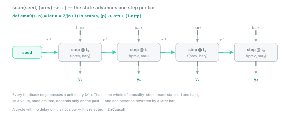 Figure —
 scan unrolled: the feedback edge always crosses a unit delay, and each emitted value is final.
The canonical example — an exponential moving average built from first principles:
def ema0(s, n) =
  let a = 2 / (n + 1) in
  scan(s, (prev) -> a * s + (1 - a) * prev)   // α → α : Σλ=1 affine step, kind-preserving
A running extreme is a one-liner:
peak = scan(high, (prev) -> math.max(prev, high)) // price — running maximum since the first stepComposite state: a record seed
State rarely stays scalar. Seed a scan with a record and the whole record is the
accumulator; the kind system tracks every field.
dd = scan({ peak: close, draw: 0 }, (prev) ->
  let p = math.max(prev.peak, close) in
  { peak: p, draw: (p - close) / p })         // record{peak: price, draw: ratio}
plot dd.draw                                  // (p − close) : level ; level ÷ price → ratio
A trailing-stop with a flip — the SuperTrend family — is a record of a price and a dir
({-1, 0, +1}, compared with ==, never matched):
def flip(mult) =
  let band = mult * atr(14) in                // num × level → level
  scan({ stop: close - band, side: 1 }, (prev) ->
    if prev.side == 1 then
      if close < prev.stop then { stop: close + band, side: -1 }
      else { stop: math.max(prev.stop, close - band), side: 1 }     // ratchet: never loosens
    else
      if close > prev.stop then { stop: close - band, side: 1 }
else { stop: math.min(prev.stop, close + band), side: -1 })State machines: a variant seed and match
When state is a mode, seed the scan with a variant and step it with match — the
eliminator forces every mode to be handled ([ErrTotalMatch] otherwise), so a state machine
cannot silently forget a case:
variant Phase { Flat | Long(entry: price) }

def step(prev) = match prev {
  Flat    -> if close cross_up ema(close, 50) then Phase.Long(entry: close) else Phase.Flat
  Long(e) -> if (e - close) / e > 0.05 then Phase.Flat else prev
}

pos = scan(Phase.Flat, (prev) -> step(prev))
Look at the exit rule, because the kind system wrote it. The obvious first draft is
close < e * 0.95 — and it is rejected: e is a price, an affine point, and scaling a
point by a scalar has no meaning (5% of “the 42nd parallel” is not a place). The algebra erases
the dimension, and comparing the result back against a price is [ErrDim]. What you actually
meant is a displacement measured against the entry — (e - close) / e, a price − price
over a price, which is a ratio, and a ratio compares with 0.05 happily. The compiler did
not merely refuse the first draft: it named the second.
Worked sketch: a point-and-figure column
Price-driven representations keep a column state: which way the column runs, its running
extreme, how many boxes it has filled. As scan state:
// state : record{ dir: dir, extreme: price, count: num }
def pnfCol(box, rev) =                        // box : level (const-folded), rev : num
  scan({ dir: 1, extreme: close, count: 0 }, (prev) ->
    if prev.dir == 1 and close >= prev.extreme + box then
      prev with { extreme: prev.extreme + box, count: prev.count + 1 }
    else if prev.dir == 1 and close <= prev.extreme - rev * box then
      { dir: -1, extreme: prev.extreme - rev * box, count: rev }
    else prev)                                // sketch: up-side only, one box per step
The kinds are the point of the sketch. count is a pure number of boxes — dimensionless —
while box : level carries the price dimension. So:
count * box : level— a number of boxes times a box height is a displacement;extreme + count * box : price— anchoring that displacement at the column’s extreme gives back a point on the price axis.
Store count : num and the algebra reconstructs every geometric quantity with the right
kind; store a price per box and the arithmetic would type as nonsense (price + price has no
affine meaning). The production version of this sketch is not a scan at all but a change of
clock — pnf(box, rev) in Clocks — yet its internal
state types by exactly this reasoning.
stateful — the low-level escape hatch
stateful(seed, (st, bar) -> e) exposes the engine’s recursive primitive directly: you
receive the previous state and the current step’s raw data, and return the next state. It is
the same construct as scan with the sugar removed, for the rare kernel whose step cannot be
phrased as an expression over named streams. Prefer scan; reach for stateful when you
need the whole bar record at once.
acc = stateful({ n: 0, ups: 0 }, (st, bar) ->        // seed is a RECORD; bar is the whole step
{ n: st.n + 1, ups: st.ups + (if bar.close > bar.open then 1 else 0) })loop — bounded iteration within a step
loop(max, init, step) iterates within a single step: max rounds (const-folded), starting
from init and applying step to the running value. It is the total replacement for a while:
the bound is part of the program, so termination is a fact, not a hope. Root-finders,
implied-value solvers and smoothing passes are its natural users.
def nroot(x) =                                // num → num : Newton, a fixed 24 rounds
  loop(24, x / 2, (g) -> (g + x / g) / 2)

plot nroot(rsi(close, 14))                    // dimensionless in, dimensionless out
Totality comes from max, and from max alone. It is a static ceiling: the compiler budgets
the worst case, so the cost of a step is known before the step runs, whatever the data does. In
this shipped form the ceiling is also the exact count — loop runs max rounds and takes the
last value — which in practice costs nothing here, because Newton doubles its correct digits each
round: an f64 root has converged long before round 24, and the remaining rounds are fixed
points.
The sealed design carries a fourth argument, an early-exit predicate:
loop(max, init, step, until) stops as soon as until holds. That does not weaken totality —
the budget is still max, and the compiler still reserves it — it only lets a converged iteration
stop paying for rounds it does not need. The shipped signature does not take it yet, so the form
above is the one that runs today.
No unbounded loop exists in the v1 surface: there is no token for one, and every practical
iterative kernel states its budget. (The design weighs an opt-in unsafe escape for an unbounded
loop and turns it down by default; nothing in the catalogue needs one.)
Cumulative and anchored streams
Two combinators cover “since forever” and “since an event”:
cum(x) → α— the expanding sum from the first step (ascanin a coat);cumSince(reset, x) → α— the same accumulation, re-initialized at each rising edge of thereset : signal.
total = cum(volume)                                        // volume — since the first step
sess  = in_session("09:30-16:00 America/New_York")         // signal — 1 while the session is open
sVol  = cumSince(sess, volume)                             // volume — since the session opened
The anchored VWAP is this idiom applied to a ratio of accumulations — and it types because the dimensional algebra divides the dimensions out:
sess  = in_session("09:30-16:00 America/New_York")                // signal — the anchor
avwap = cumSince(sess, close * volume) / cumSince(sess, volume)   // pv ÷ volume → price
// packaged later: avwap = vwap(anchor: sess)
Any signal can anchor: a session open, a crossover, a structural break. An input of kind
price or time may be placed by click on the chart — the host writes the chosen value
back as a pinned input, so the analysis still reads an input, never the pointer, and a
“VWAP since the step I clicked” stays fully causal and replayable.
Clocks: the step axis is a value
Every series advances on a clock, and clock is a first-class kind: an ordinal step
index plus a mapping between step indices and time. A clock answers two questions — what is
step i’s timestamp? and which step contains time t? — and nothing else; position on
the axis is always the ordinal index, never wall-time.
Four constructors build clocks:
| constructor | steps advance on | example |
|---|---|---|
tf("1h") |
closed time buckets | hours, days, weeks |
renko(box) |
price moving one box : level |
bricks |
pnf(box, rev) |
price filling boxes, reversing after rev |
point-and-figure columns |
range(r) |
price traversing a range r |
range bars |
Time-coarse clocks and price-driven clocks are the same concept: a rule for when a unit closes. This is why alternative chart representations are not renderers bolted onto bar data — a Renko or point-and-figure series is the ordinary series machinery running on a different clock — and why multi-resolution analysis is not a special feature: an expression at another resolution is an expression on another clock, resampled back (next section).
Clocks are ordinary values. They flow through if, through def parameters, through
input:
regime = adx(14).adx > 25                     // signal — a trending regime
c      = if regime then tf("1d") else tf("4h") // clock — chosen like any other value
Constructor parameters const-fold: renko(50) (the literal adopts kind level), or a
bounded input. A data-dependent box is rejected — a clock is a fixed axis, not a quantity
that drifts with the data it is supposed to index.
Functions may consume clocks like any value: barsPerYear(clk) → num derives the
periods-per-year of a time clock (for annualization); on an event clock (renko, pnf) the
question has no answer and it returns na with a diagnostic.
@ — the clock eliminator
e @ c evaluates e per unit of the clock c and reads the result back on the current
series’ steps. It is the eliminator of the clock kind — clocks are outside arithmetic,
and @ is the one operation that consumes them. Resampling is kind-preserving
(resample : (α, clock) → α) and causal: at any step, e @ c reads the value of e at
the last closed unit of c — never the forming one.
c   = tf("4h")                                // clock — a first-class value
d   = ema(close, 20) @ "1d"                   // price — the daily EMA, on the chart's steps
r   = rsi(close, 14) @ tf("1h")               // osc(0,100) — kind-preserving
x   = close @ c                               // any clock value works as the operand
The operand may be a string literal (shorthand for the time-coarse clock it names), an identifier
or a call (tf("1h"), renko(box)), or a parenthesized expression. @ is a postfix operator and binds tighter than
comparison, which makes the confluence idiom read naturally:
plot close > ema(close, 20) @ "1d" // signal — close vs the last CLOSED daily EMAparses as close > (ema(close, 20) @ "1d"): the current step’s close against the daily
average as of the most recent completed day.
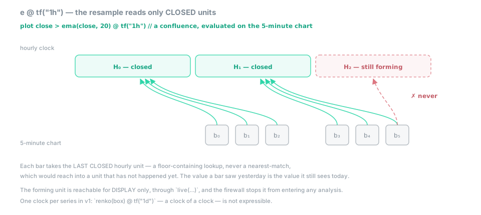 Figure —
 e @ tf("1h"): every fine step reads the last closed coarser unit; the forming unit is invisible to analysis, and steps before the first closed unit read na.
The locator is floor-containing
Mapping a step’s time t to a unit of the coarser clock uses the floor-containing rule: the
unit whose span contains t — the most recent one whose start is Tₖ ≤ t, never a
round-to-nearest match. Reading it then follows the closed-unit rule above: a step inside a
still-forming unit takes the last unit already closed.
Why this rule exists. Round-to-nearest maps a step in the first half of a forming unit to that forming unit — a value that will still change — which is a look-ahead: the analysis would read data that did not exist at the step being computed, and history would repaint when the unit closes. Floor-containing is the unique alignment under which
output[t] = f(inputs[0..t])survives resampling.
Before the first closed unit of the coarser clock, e @ c is na — resampling inherits
warm-up like everything else, and byte-identity holds through it.
The clock contract
The resampling machinery is pinned by seven invariants; they are the reference semantics of
@ and of clocks generally:
| invariant | statement |
|---|---|
| I1 | Position is ordinal — a series is addressed by step index; wall-time never enters the axis. |
| I2 | The resample locator is floor-containing — never round-to-nearest. |
| I3 | Only closed units are readable; the forming unit is invisible to ANALYSIS. |
| I4 | The time grid is the clock’s real one, not an idealized uniform grid. |
| I5 | One clock per series (v1) — clock composition is rejected. |
| I6 | Byte-identity, warm-up included: a resampled kernel matches the native one from the first step. |
| I7 | The interpreter and the compiled engine produce identical bytes, verified at every compilation. |
I5 is the honest v1 limit: a series has exactly one clock, so a clock cannot be resampled onto another clock —
close @ renko(50) @ "1d" // ✗ — one clock per series in v1: no clock compositionis rejected. Stacked re-bucketing (price bricks, then daily aggregation of bricks) is a coherent concept and deliberately out of v1’s sealed scope.
Foreign series and the as-of rule
Resampling is one instance of a general problem: aligning a series that closes on its own
schedule onto the chart’s ordinal axis. Another asset, another venue, another session
calendar — their steps do not coincide with the chart’s. The alignment rule is the as-of
join, and it is the same floor-containing rule as @:
At chart step
t, a foreign series reads its most recent step with timestamp ≤t’s time.
Never round-to-nearest — that would peek at a foreign step that had not happened yet. During
a foreign gap (its market closed, the chart’s open), the value holds: the last known
foreign value is still the most recent one. Before the first foreign step, the value is na
— ordinary warm-up.
eth = series("ETH-USD").close                 // price[ETH,USD] — aligned as-of, holds over gaps
rel = close / eth                             // ratio — cross-rate (same quote), plottable
Because the as-of join admits no future row, the no-repaint property of the composite is
inherited outright: a cross-series indicator is exactly as replayable as a single-series one.
The kind system separately guards what you may combine — asset and currency tags on price
make price[BTC,USD] + price[ETH,USD] an [ErrDim] — see
fdk/asset-currency.md.
Points, durations, periods
Three kinds carry time itself, and the affine discipline of the price axis applies verbatim to the time axis:
| kind | role | representation |
|---|---|---|
time |
a point on the timeline | machine instant (64-bit epoch) |
duration |
a vector of elapsed machine time | exact — machine tag |
period |
a vector of calendar time | zone/DST-aware — calendar tag |
duration and period are the same dimensional object — a displacement on the time axis —
distinguished by a representation tag, exactly as f64 and decimal tag the same
numeric dimension. Both additions are point + vector → point:
age    = time - time[1]                       // duration — pt(T) − pt(T) → vec(T), exact
expiry = time + time.months(3)                // time — calendar arithmetic, DST-aware
later  = time + time.months(1) + time.days(10)   // period constructors compose
period values are built only by the constructors time.years(n), time.months(n),
time.weeks(n), time.days(n) (const arguments). The two representations never mix
implicitly:
time.days(1) + (time - time[1]) // ✗ [ErrRepr] — calendar + machine: convert explicitlyWhy this rule exists. “One day” and “24 hours” are different claims: across a daylight saving transition, adding
time.days(1)lands on the same wall-clock time the next civil day, while adding a 24-hourdurationlands an hour off. Both are useful; silently conflating them is how session logic breaks twice a year. The tag keeps each addition honest and makes the conversion a visible decision.
Calendar accessors — year, month, day, hour, minute, second, dayOfWeek,
dayOfYear — project a time into a declared zone and return num. The default zone is a
pinned replay input: since an accessor runs in the ANALYSIS plane, its zone cannot be an
ambient per-viewer setting, or two machines would compute different values for the same
script; where no pinned default applies, the zone is written explicitly, as in_session
already does. Arithmetic that leaves the representable range does not wrap: it yields na
with a diagnostic, preserving the causal order of timestamps.
live(e) — the forming unit, display only
Everything above concerns confirmed values: streams that advance when a unit closes.
Displays legitimately want one more thing — the unit still forming. live(e) provides it,
as a presentation signal:
live(e)re-evaluates the analysis sub-graph ofeper frame, including the forming unit;κ(live(e)) = κ(e)— it is kind-preserving.e @ live(tf("1h"))scopes the reading to the resample: only the coarser clock’s forming unit is read live; everything else stays confirmed.- A
live(…)value may flow only into display sinks:plot,mark,fill,color bars, a scene. It is provisional by nature — each frame’s value supersedes the last, and none is committed or journaled; when the unit closes, the confirmed value takes over.
Any confirmed sink is barred by the firewall — the one-way boundary between presentation and analysis (see The four planes & the firewall):
plot live(ema(close, 20))                     // ✓ display — the forming step included, per frame
h1  = high @ live(tf("1h"))                   // ✓ display — the forming hour's running high

rsi(live(close), 14)                          // ✗ [ErrFirewall] — feeding an analysis calculation
alert live(close) > sma(close, 20)            // ✗ [ErrFirewall] — alerts are confirmed sinks
assert live(close) > 0                        // ✗ [ErrFirewall] — assertions run on confirmed data
The confirmed stream of e is untouched — byte-identical with or without live anywhere in
the script — and live() values are excluded from the byte-identity oracle exactly as
wall-clock signals are. A script that uses live() is flagged non-replayable: its
display cannot be reproduced from the journal, because the forming data it painted was never
committed. Its analysis remains replayable; the flag is about the pixels.
Why this rule exists. The forming unit is the one value in the system that will change. Letting it into a calculation would manufacture exactly the repaint the language exists to exclude — an indicator that looks prescient live and rewrites itself at the close. Routing it to display sinks only gives the legitimate use (watching the current unit develop) with zero effect on any confirmed value, any alert, any replay.
Session, event and pivot helpers
The small vocabulary that connects streams to calendars and events:
| helper | kind | meaning |
|---|---|---|
in_session(spec) |
signal |
1 while the named session is open; the spec names hours, zone and the asset calendar |
barssince(s) |
barspan |
steps elapsed since s last fired |
valuewhen(s, x) |
kind of x |
the value x had when s last fired |
count(s, n) |
osc(0,n) |
how many of the last n steps fired s |
rising(x, n) / falling(x, n) |
signal |
monotone over the last n steps |
a cross_up b / a cross_down b |
signal |
crossing, as an infix comparison |
barssince returns barspan, not a bare number: counts of steps carry the ordinal dimension
(the x-axis is affine too), so a bar count cannot be silently added to a price — while
barindex − barindex → barspan and slope-like quantities (price per barspan) fall out of
the algebra with correct kinds.
sess  = in_session("09:30-16:00 America/New_York")   // signal
sinceX = barssince(close cross_up ema(close, 50))    // barspan
atX = valuewhen(close cross_up ema(close, 50), close) // price — held until the next firingPivot confirmation: latency in the signature
A pivot — a local extremum — is only knowable in hindsight: a high is not a pivot high until
enough later steps have failed to exceed it. Flux makes that hindsight explicit. Pivot
detectors return signal @lag right: the signal fires on the step where confirmation
completes, right steps after the extremum, and the @lag annotation is part of the frozen
signature — the latency is documented, bounded and visible to the reader, not an
implementation surprise. The pivot’s value is retrieved with valuewhen:
ph  = pivot_high(high, 3, 3)                  // signal @lag 3 — confirmed 3 steps after the top
lvl = valuewhen(ph, high)                     // price — the last confirmed pivot level
The familiar alternative — a zigzag whose last leg mutates until the next pivot confirms
— is inexpressible, and deliberately so: a mutating last value means a produced value changed
(repaint, excluded by the causality theorem), and its confirmation latency is unbounded
(excluded by totality). The causal decomposition is: confirmed pivots as analysis values
(above), and — where a forming leg is wanted on screen — a provisional presentation marker
fed by live(), which never becomes an analysis value. What cannot be written is precisely
the part that would have lied.
See also
- Kinds — the dimensional kind system these streams carry: sorts, tags,
naas⊥. - Operators — the per-operator dimensional algebra,
?-family,with. - Inference — how kinds (and warm-up
na) propagate through a program. - Canvas — the frame clock, presentation signals, and where
live()values land. - compute — dataframes,
asofJoinand the windowed statistics built on these primitives. - Guide §13 — Cookbook — worked recipes: multi-resolution confluence, anchored VWAP, state machines.