Streams, delay and running state
You never write a loop, and you never manage an index — yet the indicator you wrote updates on every bar, remembers what it saw, and never once peeks at the future. That combination is the subject of this chapter. It works because a value in Flux is not a number: it is a stream, the whole history of a quantity, and the language gives you exactly three moves over it — reach a bounded distance into the past, carry running state forward, and accumulate. What it withholds is the one move that would break everything: reaching forward.
By the end you will read close[1] as “the previous close,” write a running maximum in one
line, seed a small state machine, and understand why an indicator computed live is
bit-for-bit the same indicator you scroll back to an hour later. The formal statements of all
of this live in the spec; here we build the intuition and link down.
Everything is a stream
A value in the ANALYSIS plane is a value-over-steps. close is not the last price — it is the
entire sequence of closing prices, one per step of the chart’s clock. A constant is just a
degenerate stream, the same value at every step. In the charting specialization a step is a
bar, but nothing in the model depends on that reading; a step is no more than “the next unit of
the clock.”
Because values are whole histories, arithmetic on them is element-wise: an expression relates two streams and produces a third, one relation that holds at every step at once.
fast   = ema(close, 12)      // price — a stream: one value per step
slow   = ema(close, 26)      // price
spread = fast - slow         // level — element-wise: spread at step t = fast[t] - slow[t]
There are no indices to keep straight and no loop to write. You state the relation fast - slow once, and it is understood to hold at step 0, step 1, and every step after. Under the
hood the runtime is incremental — when a new bar arrives each node advances by exactly one
step, reusing its own small pot of state; nothing is recomputed from the beginning of history.
The two ways of reading the program — as whole histories related all at once, or as one step
advancing at a time — describe the same computation, and the compiler owes you their
equivalence.
That index-free reading is not a convenience; it is the foundation the rest of the chapter stands on. A program that never names a position can never name a future position, and an operator that always advances one bounded step at a time makes termination and memory bounds properties of the language rather than of your discipline.
Reaching into the past: x[n]
The one way to look backward is the postfix delay x[n] — the value the stream x held n
steps ago.
prev = close[1]              // price — the previous step's close; na on the first step
diff = close - close[1]      // price − price → level : the one-step change
up4  = close > close[4]      // signal — na on the first four steps (comparison propagates na)
Read close[1] as “close, one step back.” Notice the second line types as a level, not a
price: subtracting one point on the price axis from another gives a displacement, and the
kind system tracks that for you (Guide chapter 5 tells that story in full).
A delay is memory, and memory is bounded at compile time, so the index obeys two rules. It
must be a const-folded constant with n ≥ 0 — a literal, or a parameter whose bounded
range lets the compiler reserve the worst case. And a delay you cannot bound is rejected
outright:
k = barssince(close cross_up open)
close[k]                     // ✗ [ErrTotal] — the lag must be a compile-time constant
k depends on the data — it could be any number of steps — so close[k] would ask the
runtime to remember an unbounded amount of history, and the compiler refuses it with
[ErrTotal]. Before step n there is no value to return at all: x[n] reads na, the
absent value, which the next section handles properly.
There is no “next value”
x[-1] — the value one step ahead — does not exist. Not as a discouraged form, not as a
lint a determined author can switch off: there is no such form in the grammar. The delay index
is non-negative by the definition of the language, and writing a negative one is an error.
close[-1] // ✗ [ErrCausal] — the future is not addressableWe make causality a compile-time property rather than a style rule for a concrete reason. In a
language where x[-1] parses and merely warns, every guarantee downstream — that a replay
reproduces the past, that an alert means what it says, that a re-run yields the same bytes —
holds only for the scripts that happened to behave. Flux inverts the burden: the misbehaving
script is inexpressible, so the guarantees hold for every program that compiles at all.
Causality is a theorem, not a promise
Put those two facts together — the past is reachable only through bounded, non-negative delay, and the currently-forming unit of any clock is unreadable — and something strong falls out. By construction, every ANALYSIS program satisfies:
output[t] = f(inputs[0..t])The value at step t is a function of the inputs up to and including t, and of nothing
later. Two consequences matter to you daily.
A feedback loop must cross a unit delay. A definition may depend on its own previous value — that is precisely what running state is — but never on its own current value. A cycle with no delay has no causal reading, so it is rejected:
ema20 = 0.1 * close + 0.9 * ema20                       // ✗ [ErrCausal] — cycle with no unit delay
ema20 = scan(close, (prev) -> 0.1 * close + 0.9 * prev) // ✓ the delay is built into scan
The fix is not to insert a delay by hand but to use scan, the sanctioned way to close a
loop, which hands you the previous step’s output so the unit delay is part of its meaning. We
come back to it below.
No-repaint. Since output[t] depends only on inputs[0..t], and inputs only ever get
appended to, a value once produced can never be contradicted by later data. This is the
no-repaint guarantee, stated plainly: a value, once produced for a step, never changes.
The chart you scroll back to is exactly the chart that was computed live; the alert that fired
is exactly the alert a re-execution fires. Repaint is not detected or warned about — it is
absent from the vocabulary. The whole family of rejections that protect this — a negative
delay, a non-causal resample, a feedback cycle with no unit delay, an unbounded lag — shares
one diagnostic: [ErrCausal].
Warm-up and na
Most kernels need some history before they can answer honestly: a 14-step RSI has nothing true
to say at step 3. Until enough data has arrived a kernel’s output is na, the absent value.
That is its natural warm-up, and each kernel inherits exactly the warm-up of its own
definition — the language does not bolt a blanket “na until N” policy on top. Determinism
holds from the very first step: a Flux kernel and the host’s native implementation of the same
kernel produce the same numbers on every machine, warm-up included.
na lives in every kind and flows through arithmetic with the kind preserved. Its comparison
rules are strict, and this trips people up once, so learn it once:
r     = rsi(close, 14)       // osc(0,100) — na on steps 0..13
warm  = is_na(r)             // signal — 1 during warm-up
bad   = r == na              // na, always — never true; use is_na
assert r <= 100              // passes from step 0: na <= 100 is na, and an na verdict is PASS
Any comparison touching na — na == x, na < x, even na == na — is itself na, never
true or false. You therefore cannot test absence with ==; you test it with
is_na(x), and its dual is_some(x) for presence. The assert on the last line is
worth dwelling on: an assertion fires only on a signal that is definitively false, and an
na verdict counts as PASS, so warm-up can never produce a spurious failure. When absence
itself should fail, you spell it out: assert is_some(r) and r <= 100.
To substitute a default, use nz(x, d), or its operator form x ?? d — the same construct
written two ways:
o  = nz(obv(), 0)            // volume — 0 is a literal and adopts the slot's kind
f  = close ?? sma(close, 5)  // price — x ?? d ≡ nz(x, d); right-associative
Both operands must agree dimensionally — the result kind is their join — and matching the
dimension but not the representation (an f64 against a decimal, machine time against
calendar time) is [ErrRepr], a request for an explicit conversion.
One asymmetry is worth memorizing because it is easy to assume wrongly. Arithmetic
propagates na, but three pointwise operators absorb it — math.max, math.min, nz — so
math.max(x, na) = x and a missing operand does not poison a running extreme. Window
reducers do not inherit that absorption: highest(x, 20) over a window with a hole in it
yields na, exactly as sma, sum and stdev do. That split is deliberate and pinned to
the native host kernels: the window reducers follow the oracle, so a hand-written fold using
max (which skips na by absorption) is a different, legitimate program — not a faster
spelling of highest.
Windows and bounded iteration
When you need more of the past than a single delay, window(x, n) materializes the last n
values of a stream as a vector — at every step.
w = window(close, 20) // vec(price, 20) — the last 20 closes, at every stepThe capacity n is const-folded, just like a delay index: a literal, or an input with a
bounded range so the compiler can reserve the worst case. A capacity that drifts with the data
is rejected for the same reason close[k] was:
len = barssince(close cross_up open)
window(close, len)           // ✗ [ErrTotal] — capacity must be a compile-time constant
Over a window you get the total for-loop. fold and map visit exactly the window’s
capacity, no more and no fewer, so they terminate by construction:
w    = window(close, 20)
hi   = w.fold(na, (acc, x) -> math.max(acc, x))   // price — max absorbs na during warm-up
devs = w.map((x) -> x - sma(close, 20))      // vec(level, 20) — element-wise, kind-tracked
Notice fold seeding with na and folding with math.max: because max absorbs na, the
warm-up holes drop out of the running maximum, and you get a clean answer even before
the window has filled.
![x[1] shifts a stream by one step; window(x,4) slides a capacity-4 vector, both na-padded during warm-up](../assets/delay-window.svg) Figure — the delay
Figure — the delay x[1] and the window window(x, 4) on one series: the past that does not exist yet reads as na.
Why there is no filter
Reach for the operation you know from other languages and it is missing:
w.filter((x) -> x > 0) // ✗ — there is no filter: the result length would depend on dataA filter’s output length depends on the data, and a flatMap multiplies lengths by a
data-dependent factor. Neither has a compile-time capacity — and capacity is exactly what
carries the totality and memory guarantees, since every collection in Flux is a vec<κ>[n]
whose n is a bound the compiler can charge against its budget. So selection never shrinks
a collection; it masks it, keeping the shape and marking the misses:
vec.where(v, pred)— same length,nawhere the element fails the predicate;vec.mask(v, live)— same length,nawhere the parallelsignalvector is 0.
w     = window(close, 50)                          // vec<price>[50]
above = vec.where(w, (x) -> x > sma(close, 50))    // vec<price>[50] — na holes, no shrinking
Masked vectors then compose with na-aware iteration: a hole produces nothing. Folds and
reducers see the na and apply their own policy; a view or canvas comprehension skips it
entirely, so a masked-out element draws no child:
group { for lvl in window(close, 5) -> dot { at:(bar.i, lvl) } } // na elements: no dotThe reasoning behind all of this is one sentence: “bounded memory” is only a theorem if no
operation can grow a collection past its declared capacity or make its size a runtime
surprise. Masks keep the shape static and move the “how many survived?” question into the
values — the na holes, a count where you need one — which is exactly the information a
total program is free to carry.
Running state: scan
scan(seed, (prev) -> e) is the running accumulator, and it is the language’s feedback
construct. At the first step, prev is the seed; at every step after, prev is the value the
scan itself produced one step earlier. The emitted value is the state. The unit delay that
causality demands lives inside the combinator — prev is always one step old — so a scan can
never read its own current output, and you never have to remember to insert the delay
yourself.
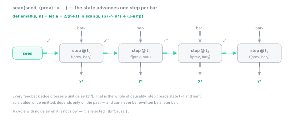 Figure —
 scan unrolled: the feedback edge always crosses a unit delay, and each emitted value is final.
An exponential moving average built from first principles is the canonical example:
def ema0(s, n) =
  let a = 2 / (n + 1) in
  scan(s, (prev) -> a * s + (1 - a) * prev)   // α → α : Σλ=1 affine step, kind-preserving
Each step blends the current input with the previous output; the weights sum to one, so the step is affine and the kind flows straight through. A running extreme is even shorter:
peak = scan(high, (prev) -> math.max(prev, high)) // price — running maximum since the first stepState that is a record
State rarely stays a single scalar. Seed a scan with a record and the whole record becomes
the accumulator, with the kind system tracking every field. Here is a running drawdown — the
peak seen so far, and how far below it price sits now:
dd = scan({ peak: close, draw: 0 }, (prev) ->
  let p = math.max(prev.peak, close) in
  { peak: p, draw: (p - close) / p })         // record{peak: price, draw: ratio}
plot dd.draw                                  // (p − close) : level ; level ÷ price → ratio
The kinds do bookkeeping you would otherwise do in your head: p - close is a level, a
displacement, and dividing it by a price gives a dimensionless ratio — exactly what a
drawdown is. A trailing stop with a flip, the SuperTrend family, is the same idea with a
direction field carried alongside the price:
def flip(mult) =
  let band = mult * atr(14) in                // num × level → level
  scan({ stop: close - band, side: 1 }, (prev) ->
    if prev.side == 1 then
      if close < prev.stop then { stop: close + band, side: -1 }
      else { stop: math.max(prev.stop, close - band), side: 1 }     // ratchet: never loosens
    else
      if close > prev.stop then { stop: close - band, side: 1 }
      else { stop: math.min(prev.stop, close + band), side: -1 })
The side field is a plain {-1, 0, +1} direction, compared with ==; the math.max /
math.min on the held side is the ratchet that keeps the stop from ever loosening.
State that is a mode: match
When the state is a mode rather than a number, seed the scan with a variant and step it
with match. The eliminator forces you to handle every mode — [ErrTotalMatch] if you forget
one — so a state machine cannot silently drop a case:
variant Phase { Flat | Long(entry: price) }

def step(prev) = match prev {
  Flat    -> if close cross_up ema(close, 50) then Phase.Long(entry: close) else Phase.Flat
  Long(e) -> if (e - close) / e > 0.05 then Phase.Flat else prev
}

pos = scan(Phase.Flat, (prev) -> step(prev))
Look closely at the exit test, because the kind system wrote it for you. The obvious first
draft is close < e * 0.95, and Flux rejects it: e is a price, an affine point, and
scaling a point by a scalar is meaningless — 5% of “the 42nd parallel” is not a place. So the
algebra erases the dimension, and comparing the result back against a price is [ErrDim].
What you actually meant is a displacement measured against the entry — (e - close) / e, a
price − price over a price, which is a ratio, and a ratio compares with 0.05 happily.
The compiler did not merely refuse the wrong version; it pointed at the right one.
A worked sketch: a point-and-figure column
Price-driven chart representations keep a small column state — which way the column runs, its
running extreme, and how many boxes it has filled. As scan state that reads:
// state : record{ dir: dir, extreme: price, count: num }
def pnfCol(box, rev) =                        // box : level (const-folded), rev : num
  scan({ dir: 1, extreme: close, count: 0 }, (prev) ->
    if prev.dir == 1 and close >= prev.extreme + box then
      prev with { extreme: prev.extreme + box, count: prev.count + 1 }
    else if prev.dir == 1 and close <= prev.extreme - rev * box then
      { dir: -1, extreme: prev.extreme - rev * box, count: rev }
    else prev)                                // sketch: up-side only, one box per step
The kinds are the whole point of the sketch. count is a pure number of boxes —
dimensionless — while box : level carries the price dimension, so count * box is a
displacement and extreme + count * box is a point back on the price axis. Store count : num and the algebra reconstructs every geometric quantity with the right kind; store a price
per box instead and the arithmetic would type as nonsense, because price + price has no
affine meaning. In production this is not a scan at all but a change of clock — the same
column logic expressed as pnf(box, rev), which Guide chapter 6 covers — yet its internal
state types by exactly this reasoning.
The lower-level tools
Two escape hatches sit underneath scan, for the rare step it cannot phrase.
stateful(seed, (st, bar) -> e) exposes the engine’s recursive primitive directly: you get
the previous state and the current step’s raw bar, and you return the next state. It is scan
with the sugar removed, for a kernel whose step needs the whole bar record at once rather than
a named stream:
acc = stateful({ n: 0, ups: 0 }, (st, bar) ->        // seed is a RECORD; bar is the whole step
  { n: st.n + 1, ups: st.ups + (if bar.close > bar.open then 1 else 0) })
loop(max, init, step) iterates within a single step — max rounds, const-folded, starting
from init. It is the total replacement for a while: the bound is part of the program, so
termination is a fact rather than a hope. Root-finders and smoothing passes are its natural
users:
def nroot(x) =                                // num → num : Newton, a fixed 24 rounds
  loop(24, x / 2, (g) -> (g + x / g) / 2)

plot nroot(rsi(close, 14))                    // dimensionless in, dimensionless out
Totality comes from max, and from max alone. It is a static ceiling: the compiler budgets
the worst case, so the cost of a step is known before the step runs, whatever the data does.
In the shipped form the ceiling is also the exact count — loop runs max rounds and takes
the last value — which costs nothing in practice here, because Newton doubles its correct
digits each round: an f64 root has converged long before round 24, and the remaining rounds
are fixed points.
The sealed design carries a fourth argument, an early-exit predicate:
loop(max, init, step, until)stops as soon asuntilholds. That does not weaken totality — the budget is stillmaxand the compiler still reserves it — it only spares a converged iteration the rounds it does not need. The shipped signature does not take it yet, so the three-argument form above is the one that runs today.
This is the honest shape of Flux’s totality, and it is worth naming plainly: the work per step is bounded, knowable and compile-counted, while a stream is unbounded over time — it runs as long as bars keep arriving. That is the deliberate synchronous-dataflow trade Flux takes from the Lustre/Esterel family, not a missing feature. In a client-side reactive domain it costs you nothing you would want: an unbounded inner loop there is just a hung tab, i.e. a bug. Guide chapter 14 lays out where the trade is felt and where it is invisible.
Cumulative and anchored streams
Two combinators cover the two most common accumulations — “since forever” and “since an event”:
cum(x)— the expanding sum from the first step (ascanin a coat);cumSince(reset, x)— the same accumulation, re-initialized at each rising edge of areset : signal.
total = cum(volume)                                        // volume — since the first step
sess  = in_session("09:30-16:00 America/New_York")         // signal — 1 while the session is open
sVol  = cumSince(sess, volume)                             // volume — since the session opened
The anchored VWAP is this idiom applied to a ratio of two accumulations, and it types cleanly because the dimensional algebra divides the dimensions out:
sess  = in_session("09:30-16:00 America/New_York")                // signal — the anchor
avwap = cumSince(sess, close * volume) / cumSince(sess, volume)   // pv ÷ volume → price
// packaged later: avwap = vwap(anchor: sess)
Any signal can anchor — a session open, a crossover, a structural break. And an input of
kind price or time can be placed by click on the chart: the host writes the chosen value
back as a pinned input, so the analysis still reads an ordinary input rather than the pointer,
and “VWAP since the bar I clicked” stays fully causal and replayable.
See also
- Guide §5 — Kinds — the dimensional kinds these streams carry, and why
price − priceis alevel. - Guide §6 — More than one clock — clocks as values,
@resampling, foreign series, andlive(). - Guide §14 — What Flux deliberately doesn’t do — the honest shape of totality and the not-Turing-complete trade.
- Spec — Time & state (Analysis) — the reference semantics narrated above.
- FDK — Compute — dataframes,
asofJoin, and the windowed statistics built on these primitives. - Guide §13 — Cookbook — worked recipes: anchored VWAP, state machines, running state.
The formal rules →
Everything this chapter narrated is specified exactly in Time & state (Analysis):
- The stream model and element-wise arithmetic →
- The delay operator
x[n], and why there is no negative index →- Causality as a theorem, and the no-repaint guarantee →
- Warm-up,
na, and absorption vs propagation →- Windows,
fold/map, and masking (where/mask) →scan,stateful,loopand running state →cum,cumSinceand anchored streams →