#Your first session

You have seen why Flux is built the way it is; now watch those guarantees from the keyboard. The fastest way to feel what Flux is for is to write one line and watch how much it decides on your behalf. This chapter is a guided first session: it starts with the shortest program that does something real and grows it — a parameter, some styling, a function you compose out of smaller ones — narrating what the language did for you at each step and, just as tellingly, what it declined to do.

The examples here are all financial charting, the flagship domain — but the kind-and-stream machinery they show is general, and holds for any bounded causal series: a sensor trace, a log, a game’s turns.

Everything here is a complete program. Paste any of it into the editor and it runs.

#One line

This one line is a complete, publishable analytic — and it is live. Edit it right here and it recompiles and re-renders in your browser as you type: change the 14, swap rsi for ema or sma, or drop the input(…) wrapper entirely and watch the parameter knob disappear.

plot rsi(close, input(14, 2..50, title: "Length"))

You configured nothing, and yet a whole chart came back — the kind of the expression carried the pane, the scale, the guides and the colour:

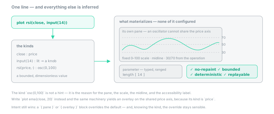Figure — one source line; the kind decides the rest.

• close is a price. rsi is a bounded oscillator family, so the expression has kind osc(0,100).
• Because the kind is a bounded oscillator, it cannot share the price axis — it gets its own pane, with a fixed 0–100 scale and a midline. Because the operation is specifically rsi, its conventional 30/70 guides are drawn too.
• Because you wrote input(14), a parameter control appears, typed and ranged.
• Because the program is causal and total by construction, it is also replayable, bounded, and byte-identical on every engine — which the guarantees panel tells you without being asked.

Delete the wrapper and write plot rsi(close, 14): the same analytic, now with no control. The input(…) wrapper is nothing more than how a value becomes a knob.

What just happened. You did not choose a pane, a scale, a colour or a reference line. The kind of the expression carried all of it. This is the single biggest ergonomic consequence of a dimensional type system, and it holds for everything you write next.

#Parameters and styling

input accepts a default, an optional range, and optional metadata:

len  = input(14, 2..200, title: "Length")
src  = input(close, title: "Source")
show = input(true, title: "Show band")

plot rsi(src, len)

The kind of the default decides the widget. A number gives a numeric field — and a range makes it a slider; close gives a source picker; true gives a checkbox; a list of strings gives an enumeration. You never wire a control to a variable; you write the value you mean, and the control is inferred from its kind.

Presentation defaults are inferred the same way, but your intent always wins:

m = macd(close)
plot m.hist { style: histogram, color: if m.hist > 0 then up else down }
plot m.macd, m.signal
plot ema(close, 200) { overlay }        // it is already a price — this is explicit
plot rsi(close, 14) { guides: [20, 80] } // your own reference lines, kind-checked

The style values are a closed set (histogram, columns, stepline, area, circles, cross); a plain line is the default that a level or a price infers. Forcing a level onto the price chart with { overlay } gives it its own secondary axis — the compiler knows a shared price scale would flatten it to nothing, so it opens one rather than draw you something useless.

And it runs live — retune the three MACD lengths below and watch the oscillator pane recompute, the signal line cross the MACD, and the histogram flip sign:

plot macd(close, input(12, 2..40, title: "Fast"), input(26, 2..80, title: "Slow"), input(9, 2..40, title: "Signal"))

#Composition

def defines a pure function from streams to streams. It is inlined into the graph, so there is no call cost to weigh:

def zscore(x, n = 20) = (x - sma(x, n)) / stdev(x, n)

plot zscore(close)          // (price − price) ÷ level = level ÷ level → ratio
plot zscore(hlc3, 50)       // the same def on another price source — the kinds follow the argument

Any function can also be written as a method-style chain, where the receiver becomes the first argument — which is how most people end up writing analytics:

smoothRsi = close.ema(20).rsi(14)     // ≡ rsi(ema(close, 20), 14)

The payoff is not brevity. After you type close., the editor offers only the functions whose first parameter accepts a price — so the type system doubles as a discovery mechanism, and the wrong composition never reaches your fingers.

Several kernels return a record, and you project the field you want:

bb = bollinger(close, 20, 2)
plot bb.upper, bb.middle, bb.lower
fill bb.upper..bb.lower      // a band: both operands are `price`, so the fill is well-formed

Write fill bb.upper..rsi(close,14) instead and you get ✗ [ErrDim] — you cannot shade the region between a price and a dimensionless oscillator, and the language says so at compile time rather than drawing you nonsense.

#What the editor is doing while you type

None of this is a build step you wait on. As you type, the editor filters completion by kind after ., shows a hover card with the signature and a live sparkline of the expression on the current data, and offers diagnostics with quick-fixes. A preview re-evaluates the typable part of your program on every keystroke — a half-typed name blanks the one value it belongs to, never the whole screen — and a dataflow view can answer “why is this signal true here?”. Working in the editor covers all of it.

#Where the session goes from here

Those three moves — write the expression, expose a knob, compose it — are the whole first arc, and the rest of the Guide grows the same program:

• A comparison such as close cross_up ema(close, 50) produces a signal, which shows as marks and alerts, never a line. See Signals, marks and alerts.
• When a value depends on its own past, you don’t loop over bars — you write a scan, a seed plus a step that receives the previous state. See Streams, delay and running state.
• Reading an expression on another clock with @ tf("1h") is the confluence idiom, and it is just an ordinary causal resample. See More than one clock.
• A moving scene lives on its own plane where every property is a signal, so there is no animation API to learn — and the scene may read your analysis while analysis can never read the scene. See A scene that moves.
• A small application adds persistent state and default-deny capabilities: a model, a pure update, a pure view, and declarative subscriptions, with every ambient thing arriving as a message. See Building an application.

Each is a plane of the same language, separated by a firewall that keeps decoration from ever touching a number — the subject of The four planes.

#See also

• Kinds — types that carry meaning — the type system that produced every default above.
• Streams, delay and running state — scan, delays and warm-up.
• Working in the editor — completion, live preview and the dataflow view in full.
• Cookbook — recipes that run — working recipes across every plane.
• FDK overview — the libraries behind rsi, macd and bollinger.

The formal rules →

• Spec · Kinds — the kind catalogue and the osc interval lattice — where price, level and osc(0,100) come from.
• Spec · Inference — presentation is inferred, not configured and the error policy — the pane/scale/style table and [ErrDim].
• Spec · Grammar — ANALYSIS sinks and parameters, the single arrow and the postfix chain — plot, input, def and method-style calls.
• FDK · overview — the prelude — the kernels in scope without an import.