#Kinds — types that carry meaning

Ask a spreadsheet what close − open is and it answers “a number.” Ask Flux, and it answers something sharper: a level — a displacement along the price axis, a different animal from close itself, which is a price, a point on that axis. Every value in Flux carries a kind: a statement of what it means, not merely how it is stored. rsi(close, 14) is not a float that happens to sit between 0 and 100 — it is a bounded oscillator, osc(0,100). Once meaning rides along with the value, three chores you would otherwise do by hand happen on their own. The compiler refuses arithmetic that has no meaning. It reconciles the branches of an if and the series you co-plot without you spelling out the rule. And it lays out the chart for you, because a value that knows it is a bounded oscillator already knows it wants its own 0–100 pane.

This chapter builds the intuition one idea at a time — what a kind is, why the compiler treats subtraction and reconciliation as different questions, and how the same knowledge that catches a bug also draws the pane. The machinery is general (it kinds calendar arithmetic, exact decimal money, physical units, and the App plane’s messages and views just as readily), but market data is the running illustration. The exhaustive lattice, the full catalogue and the complete presentation table are the spec’s job; you’ll find them linked at the foot of the page.

#Two questions the compiler keeps apart

First the intuition, because everything below is only this idea made precise: a kind is what a value physically is — close is a point on the price axis, close − open a displacement along it, rsi(close, 14) a bounded, dimensionless reading. That much carries on plain words. The lattice notation that follows — the join ⊔ here, the extrema ⊤ and ⊥ later — is only how the compiler makes those distinctions exact; its exhaustive form, every kind’s place in the partial order, is the spec’s, pinned in Kinds — the partial order, and a first read can lean on the words until you want it.

Here is the observation the whole system is built on. price − price = level, yet price ⊔ price = price. Subtraction and reconciliation look alike — both take two prices — but they answer different questions, and Flux refuses to conflate them.

• The algebra computes what an operation produces. + − × ÷ < > == each read the kinds of their operands and hand back a result kind, in the style of classical dimensional analysis. It can move across meanings — price − price becomes a level — or refuse outright, because a price plus a bare oscillator is not a thing.
• The join ⊔ asks a narrower question: is there one kind that covers both? It unifies the two branches of an if, the two arguments of nz, the series you drop into one pane. It never invents a result the way the algebra does; it only finds a common home, or fails to.

Both feed one error channel, written ⊤ (“any”). A ⊤ in a demanding position — an operand, a plot target, an argument — is a hard error; anywhere else it is a warning. And an operand is itself a demanding position, which is why close + rsi(close, 14) fails right at the +, whether or not anything downstream ever reads it.

fast   = volume > sma(volume, 20)

spread = close - open              // price − price → level   (algebra, system B)
line   = if fast then ema(close, 12) else ema(close, 26)
                                   // price ⊔ price → price   (join, system A)
plot spread, line

// ✗ plot close + rsi(close, 14)   — [ErrDim]: point + dimensionless has no affine meaning

Read that back: spread runs through the algebra and lands on level; line runs through the join, where two prices share the kind price; and the commented line never compiles, because the algebra has no rule for a point plus a dimensionless number.

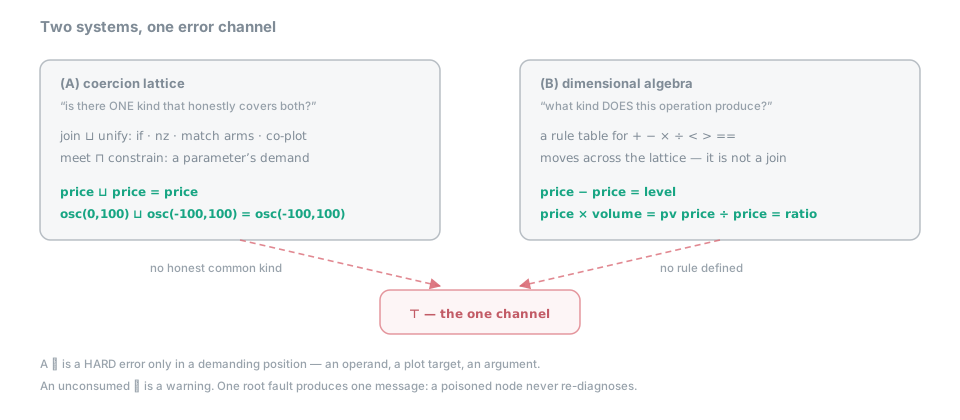Figure — the coercion lattice (A) and the operator algebra (B) meet only in the single error channel ⊤; price − price → level flows through B, never through A.

Keeping the two apart buys a distinction that is easy to miss and worth stating outright, because it separates a type system that is strict from one that is merely loud: a mixture of dimensions never reaches ⊤. Add a price to an oscillator in arithmetic and the algebra has no rule — that is a hard [ErrDim]. But reconcile a price and an oscillator by taking one branch of an if or the other, and the join does not fail. It erases the dimension and lands on quantity: a real kind, a number that remembers it is a number and has forgotten what of. The value flows, carrying a [WarnBranchDim]. The hard channel is for nonsense that is certain; the soft one for a mixture that is merely suspicious — and what separates them is not whether anything consumes the value, but where the ⊤ was born.

fast = volume > sma(volume, 20)

mix  = if fast then close else rsi(close, 14)   // ⚠ [WarnBranchDim] — no common dimension, so
plot mix                                        //   the join ERASES it: mix : quantity. It flows.

// ✗ plot close + rsi(close, 14)   — [ErrDim]: the ALGEBRA has no rule for point + dimensionless.
//                                   Hard, at the `+`, read or not: an operand is a demanding
//                                   position, and there is nothing suspicious about this — a
//                                   point plus a bare number is not a thing.
// ✗ if fast then close else up    — [ErrDim]: price ⊔ color = ⊤. Crossing SORTS is not a mixture
//                                   the lattice can erase — there is no common kind to land on.

Three lines, three fates. mix reconciles into quantity and plots, flagged. The price-plus- oscillator sum is refused at the +. And the last one is hard too, even though it is a reconciliation: a price and a color live in different sorts, share no common kind at all, and no erasure can save them. One root fault, incidentally, produces exactly one message — a ⊤ propagates as a poison that everything downstream inherits in silence, so a single typo never spills forty errors across the editor.

#Why the asymmetry is geometry

The lopsidedness of the algebra — subtraction changes the kind, addition of unlike things is banned — is not a convention someone chose. It is geometry. The price axis is a one-dimensional affine space: price is a point on it, level is a vector between points, and ratio is a dimensionless scalar. Affine geometry then hands the core rules over for free. Point − point is a vector (price − price → level). Point ± vector is a point (close + atr(14) → price). Point ÷ point is a scalar (price ÷ price → ratio). And “point + point” does not exist — which is exactly why close + rsi(close, 14) is refused rather than computed.

Above the affine pairs, × and ÷ are always well-defined: a dimension is a vector of integer exponents over the generators price, volume, time, bar-index and angle, and multiplication just adds those exponents while division subtracts them. Only +, − and the order comparisons demand equal dimension — because adding metres to kilograms, or a price to a bar count, means nothing.

gap    = close - close[1]          // level      pt(P) − pt(P) = vec(P)
band   = close + 2 * atr(14)       // price      pt(P) + lit·vec(P) = pt(P)
rel    = close / open              // ratio      P⁰ — dimensionless, centered on 1
flow   = close * volume            // pv         P·V by the group law
speed  = change(close, 5) / (5 bars)  // slope    vec(P) ÷ vec(I) = P·I⁻¹ — price per bar

Each line is the geometry doing the bookkeeping you would otherwise carry in your head: gap is a displacement, band glues a displacement back onto a point and stays a point, rel cancels the dimension away to a pure ratio, flow composes price and volume into money-flow, and speed divides a price displacement by a bar displacement to get price-per-bar — a slope, kept deliberately distinct from price-per-second. The x axis is affine too, which is why barindex − barindex is a barspan and a regression slope has a kind of its own.

#Literals fit

You do not want to annotate close + 10 to say the 10 is a price. You never have to. A const-folded literal has the kind lit, which is polymorphic in dimension — it adopts whatever kind its context supplies.

hot   = close > 30000              // price vs lit → the lit reads as price → signal
lift  = close + 10                 // lit adopts price → price
safe  = nz(change(close, 1), 0)    // level ⊔ lit = level
shift = rsi(close, 14) - 50        // osc(0,100) − lit → osc(-50,50): interval propagated

The literal takes the shape of the value beside it — a price in hot and lift, a level in safe, and in shift it even shifts the oscillator’s claimed interval down with it. Adopting a kind does not suspend arithmetic sanity, though: write rsi(close, 14) > 150 and you still get a [WarnLit], because a bounded value can never cross a bound it cannot reach.

#The kinds you’ll meet

Kinds are organised into sorts — families that join only within themselves. Inside a sort there is fine structure; across sorts there is nothing in common, so the join is ⊤. A quick tour of the ones you’ll write daily:

• The dimensionless scalars — ratio (centred on 1, multiplicative), osc(lo,hi) (bounded, the family rsi, stochastic and mfi belong to), signal (a boolean event, {0,1}), and dir (a direction, {-1, 0, +1}, the kind of a trend’s side). They all sit below num, “dimensionless of unknown role.”
• The dimensioned scalars — price and its displacement level; volume; money-flow pv; time and duration; barindex and barspan; slope; angle; and any other exponent combination the group law can produce, like price × price = P². These are pairwise incomparable — a price is not “more than” a volume — and rise not to num but to quantity, the erased dimension a lossy join produces. That gap is the single most consequential choice in the design: if a price could quietly become a num, then mixing a boolean and a price would reconcile into an ordinary plottable number and the whole point of the system would evaporate. Routing every dimensioned kind to quantity instead keeps a mixture visible and suspect, never silent.
• The categorical kinds — color, clock (a resampling schedule like tf("1d") or renko(box)), and string. Each is flat and lives outside arithmetic: you don’t compute with a colour, you consume it in a fill; you don’t plot a clock, you eliminate it with @. The one arithmetic overload in the whole categorical world is string + string, which concatenates.
• The structural kinds — vec<κ>[n], a fixed-capacity vector (the n is an upper bound, not an exact count, so a short vector fits inside a long one with its tail reading na), and record{…}, a named product. Records are load-bearing: most built-in kernels return them, which is how bollinger gives you {upper, middle, lower} and macd gives you {macd, signal, hist}.
• The App-plane kinds — variant{…}, the tagged sum an app’s messages and commands are built from, and ui, the closed set of view primitives the host renderer consumes. They join the lattice by the same construction as record, directly under ⊤, without reopening the sealed core.

Two extrema sit at the top and bottom of every sort: ⊤ (the error channel) and ⊥ (the kind of na, which inhabits every kind — absence is a value of anything). You can name and reuse structural kinds at program level:

record Band { upper: price, middle: price, lower: price }

variant Tool  { Select | Draw | Erase }
variant Save  { Saved | Failed(code: num) }

One discipline keeps these inside the guarantees: the reference graph must be acyclic. A record Node { next: Node } is rejected with [ErrTotalType], because an unbounded height would break the promise that every buffer is bounded. That same promise is why there is deliberately no function kind: lambdas are second-class, admitted only where a higher-order kernel expects one, so a value is always plain data and recursion always goes through an acyclic def or a bounded scan/loop. Flux trades general recursion for totality on purpose — the payoff is that a runaway loop is a compile error, not a hung tab.

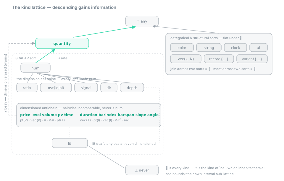Figure — the kind lattice: every sort under one ⊤ and over one ⊥; inside the scalar sort, the dimensionless spine rises to num while the dimensioned antichain rises only to quantity, and lit sits safely below every scalar.

#Presentation you didn’t configure

Now the payoff. A kind already says what a value is; so it also says how it should be shown. That is why the first program you write is one line long and needs no options at all.

plot bollinger(close, 20, 2)   // three price lines on the chart + a band — no options
plot macd(close)               // a centred pane: a histogram and a signal line
plot rsi(close, 14)            // its own 0–100 pane, midline, 30/70 guides

Each line lays itself out. The bollinger record explodes into three price fields, so they overlay on the shared price axis; macd returns level fields, so they get their own pane centred on zero; and rsi, being an osc(0,100), claims a fixed 0–100 pane, and the rsi kernel adds its conventional 30/70 guides. Nothing here was configured — the compiler derives a registry entry from the kind (pane, scale, guides, even a CSS class the host stamps on the series so a stylesheet can restyle every oscillator without naming a colour) and then refines it with metadata from the operation itself. Because inference is a deterministic function of the program, the same source yields the same kinds — and therefore the same scene — on every machine, which is what lets two engines emit the same module from it.

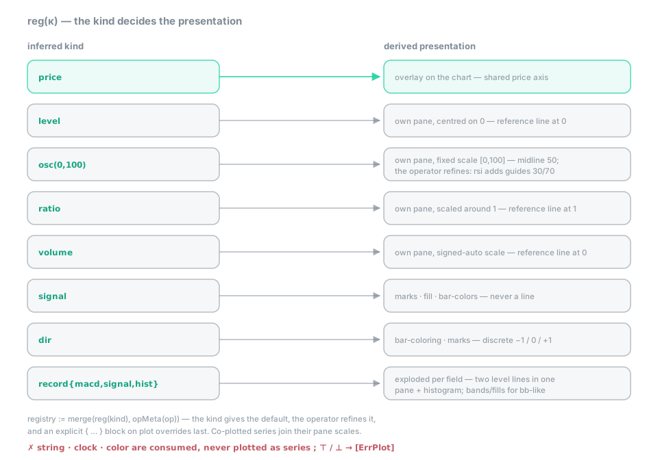Figure — reg(κ): each kind carries its own pane, scale, guides and CSS class, and the registry is merged with the operator’s own metadata. A string, a clock and a color are consumed, never plotted as a series; ⊤ and ⊥ are [ErrPlot]. None of it was configured.

Inference gives the default; you override it in the plot block, and because the system knows the kind, the override is intelligent rather than blind:

m = macd(close)
plot m.macd { overlay }                  // a level FORCED onto the chart → it gets its OWN secondary axis
plot ema(close, 20) { pane }             // a price FORCED into a pane → auto-scaled, fine

Force a level onto the price chart and the system knows a shared price scale would flatten it to nothing, so it grants a secondary axis instead of obeying you into invisibility. The same knowledge powers kind-filtered completion and the live preview: a local mistake types to a contained hole and blanks only the values that depend on it, never the whole chart — see Working in the editor.

#Meaning all the way down

Beyond its dimension, a kind can carry a few orthogonal tags — and they answer a question market data raises immediately: a price of what, in what currency, to what precision?

• A numeric representation tag: f64 by default, or exact fixed-point decimal(scale) for settled money.
• A time representation tag: machine (exact elapsed duration) versus calendar (period — a months-and-days quantity aware of zones and daylight saving).
• An asset tag (B, Q): a price is never a bare number, it is a rate, quote-per-base, and the tag carries the base and quote assets.

The tags obey two revealing regimes, and the difference between them is the whole idea. The asset tag widens on a join — reconcile two currencies and the quote component rises to a “top,” never an error — but the ± algebra demands the tags be identical, so a real unit bug is still caught at the operator:

c      = volume > sma(volume, 20)
btcUsd = series("BTC-USD").close        // price[BTC,USD]
btcEur = series("BTC-EUR").close        // price[BTC,EUR]
ethUsd = series("ETH-USD").close        // price[ETH,USD]

diff   = btcUsd - btcUsd[1]             // level[BTC,USD]
mixA   = btcUsd + ethUsd                // ✗ [ErrDim] — mixing assets
mixQ   = btcUsd + btcEur                // ✗ [ErrDim] — mixing currencies
cmpQ   = btcUsd < btcEur                // ✗ [ErrDim] — comparisons gate on identity too
rel    = btcUsd / ethUsd                // ratio — cross-base relative strength, tag dropped
either = if c then btcUsd else btcEur   // price[BTC,⊤quote] — the join widens, never errors

Subtracting BTC-USD from itself stays level[BTC,USD]; adding two different assets, or two different currencies, or comparing across them, is refused; dividing cancels the tag to a bare ratio; and reconciling in an if widens the quote instead of erroring. The representation tags, by contrast, refuse to join at all — mix an f64 price with a decimal price, in arithmetic or in a branch, and you get [ErrRepr]; the only bridge is an explicit conversion. Currency conversion needs no new machinery for any of this: fx[Q1/Q2] is just the kind ratio carrying a currency-pair annotation, and money[Q] is just decimal pv[Q] — zero new sorts, zero new lattice height. The same construction reaches past finance to physical units (meas[u] — temperatures, velocities, forces, with the same point-versus-vector discipline as price/level); the complete algebras live in units and asset & currency. (A metric[id] tag for non-price macro and on-chain series is designed and held inert — its name carried so arming it later changes no grammar.)

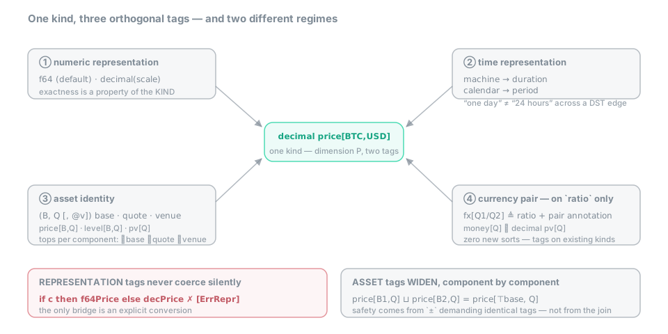Figure — the tag axes around one kind, and the two regimes: representation tags refuse to join ([ErrRepr]), asset components widen while ± demands identity ([ErrDim]).

#When the physics is wrong

Put it all together on a small chart type and watch the dimensional lens do real work. Point & Figure charting is a genuine stress test, and Flux passes it without a single new kind. The box size must be a level, because the geometry says so — it is a displacement you add to a point:

box    = atr(14)                    // level — a displacement, by construction
anchor = close                      // price — a point
edge   = anchor + 3 * box           // price ✓ — pt(P) + lit·vec(P) = pt(P)

// the column state the frontier belongs to — a plain bounded scan over a record
state  = scan({ dir: 1, extreme: close, count: 0 },
               (p) -> if close > p.extreme + box
                        then { dir: 1, extreme: close, count: p.count + 1 }
                        else p)

edge reads as “three boxes above the anchor,” and it types to a price because point plus vector is a point. Now suppose you had slipped and declared the box a price. Then anchor + box would be price + price — point plus point, no affine meaning — and the compiler stops you on the spot with [ErrDim]. The lattice does not merely permit the correct model; it refuses the incorrect one. The rest of the state types itself: count is a plain box count, deliberately not a barspan, because boxes are not bars and the kinds keep the two countings from ever being confused.

#Absence is a kind too

One last piece, because it threads through everything above: na, the absent value. Its kind is ⊥, which sits below every kind, so absence is a value of anything — never a separate shape you have to special-case. The rule that matters in practice: every comparison touching na is itself na, never true or false. So you test absence explicitly.

m   = sma(close, 200)               // price — na during warm-up
odd = m == na                       // legal, but always na — never true
hit = is_na(m)                      // signal — the way to ask
has = is_some(m)                    // signal — its dual

A 200-step average (200 bars, in charting) is na through its warm-up; comparing it to na with == gives you na, not the answer you wanted, which is why is_na and is_some exist. A NaN produced by arithmetic is na — division by zero is not an error, it is an absent value shown as a gap — and destructuring an na record hands you na in every field. Absence composes, with no special cases to memorise.

#See also

• More than one clock — clock kinds, resampling and @ in practice.
• Signals, marks and alerts — putting signal and dir to work on the chart.
• Working in the editor — kind-filtered completion, hover cards, the typable cone in live preview.
• units — the complete meas[u] algebra and affine scales.
• asset & currency — the asset tag, fx and money, venues.

The formal rules → Everything above is taught intuition; the normative statements live in the spec.

• Two systems, one error channel and the affine substrate — the algebra, the join, and why subtraction changes the kind.
• The sorts, the kind catalogue and the partial order — every kind, its dimension and its place in the lattice.
• Join and meet and orthogonal tags — the exhaustive ⊔/⊓ catalogue, representation, calendar, asset and fx tags.
• Presentation is inferred, not configured and what may be presented at all — the complete kind → registry table and the admissibility judgments.
• The error policy — every [Err…] and [Warn…] code, and what a diagnostic is.